learn · South Africa
PLC Scan Cycle Explained: Timing, Inputs and Task Order
Understand the PLC scan cycle with worked traces, missed-pulse examples and vendor I/O differences, plus practical South African training course questions.
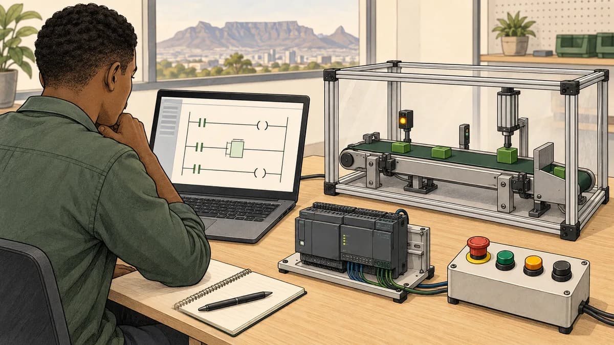
The PLC scan cycle explains when a program observes inputs, evaluates instructions and makes calculated results available. It is essential for understanding retained values, repeated execution, missed pulses and the effect of instruction order. It is also a topic where a useful beginner diagram can become misleading if it is presented as the architecture of every controller.
This tutorial starts with an explicitly simplified snapshot model. It then compares that model with documented Siemens and Rockwell behaviour, works through sequential assignments and tests a short input pulse against known sampling times. The examples use supplied values and timestamps; they are not measurements of a physical PLC.
For South African learners choosing PLC programming courses, the practical outcome is being able to explain an observed result with an execution trace. Memorising “read, execute, write” is a starting point. Knowing which data your program actually reads, and when that data can change, is the deeper skill.
Define the simplified scan model before drawing conclusions
For the first exercise, assume one repeatedly called routine with three deliberately chosen stages. First copy the supplied input into InputSnapshot. Next execute the listed statements in order, reading and writing ordinary program variables. Finally copy OutputCommand into a virtual display called PublishedOutput.
No other task interrupts this exercise. InputSnapshot remains unchanged during a routine call. Assignments to program variables take effect immediately for later statements in that call. PublishedOutput changes only at the chosen publication stage.
| Value | Meaning in this learning model |
|---|---|
| SuppliedInput | The external value offered to the model |
| InputSnapshot | The value copied at the start of the current call |
| Memory | A stored program variable retained between calls |
| OutputCommand | The program's calculated command value |
| PublishedOutput | The virtual value copied at the publication stage |
These names deliberately separate the input source, program memory and visible result. The model has no real output module or actuator. A true OutputCommand is a software value, not proof that a motor, valve or contactor has changed state.
You can draw the three stages with arrows, but write the assumptions underneath the diagram. Without those assumptions, a learner may incorrectly infer that every PLC freezes every input for an entire task or updates every output at one universal boundary.
The ladder logic basics lesson provides the Boolean background. Use this scan lesson to add time and instruction order to those Boolean expressions.
Understand process images without assuming one vendor model
A process image is a memory representation used when accessing configured input or output data. It can provide a consistent set of values for a defined portion of execution. Its update rules depend on the controller, configuration and access method.
The official Siemens S7-1200 process-image update documentation describes operating-system work, output-image transfer, input-image reading and execution of called user blocks in its stated sequence. It also identifies direct I/O access as a separate option. That is more specific than a generic drawing that always puts output transfer after the last rung.
Rockwell's ControlLogix I/O update documentation states that data updates asynchronously with logic execution. You therefore cannot assume that an ordinary I/O value read twice during a routine is necessarily unchanged between those reads.
Those sources describe different contexts. The snapshot exercise is an instructional contract, not a claim that a Siemens process image and a ControlLogix I/O tag are interchangeable. Check the exact CPU, firmware, task and I/O configuration before translating the drawing into a statement about hardware behaviour.
If a program needs a consistent local set of input values, identify the supported buffering mechanism and the required consistency scope. Copying several unrelated values with several statements does not automatically prove that they were all acquired at one physical instant.

Follow sequential assignments through one call
Consider this routine, with Memory initially false. Every statement executes on every call. OutputCommand is then copied to PublishedOutput under the simplified model.
Memory = InputSnapshot
OutputCommand = Memory
When InputSnapshot is true, the first statement writes true to Memory. The second statement reads that newly written value, so OutputCommand becomes true in the same call. It does not wait for another scan merely because Memory is a stored variable.
Now reverse the statements:
OutputCommand = Memory
Memory = InputSnapshot
The first statement now reads the value retained from the previous call. Memory still receives the current input, but the command has already been calculated. This version introduces one routine-call delay under the specified execution model.
| Call | InputSnapshot | Command: memory written first | Command: memory read first |
|---|---|---|---|
| 1 | 0 | 0 | 0 |
| 2 | 1 | 1 | 0 |
| 3 | 1 | 1 | 1 |
| 4 | 0 | 0 | 1 |
| 5 | 1 | 1 | 0 |
| 6 | 0 | 0 | 1 |
This six-call trace is more informative than saying that instructions “happen during the scan”. It identifies the exact value read at each statement. The two versions have the same assignments and different results because their order differs.
The expected table was checked in an independent software model. It is a reference for testing your own implementation, not evidence that a particular PLC project or browser runtime has been tested with these exact statements.
Use the structured text learning guide when expressing the trace as assignments. For ladder, identify the equivalent ordered networks and the storage used by each contact and coil.
Distinguish unconditional writes from conditional retention
Two unconditional assignments to one variable have a straightforward sequential result in this model. If the routine executes Command = A followed by Command = B, its final Command equals B. The earlier value may have been visible to statements between the two writes.
That is different from IF B THEN Command = FALSE. When B is false, this conditional statement performs no assignment. It does not automatically write true, and it does not automatically erase a value written earlier. The distinction matters when comparing a normal ladder output instruction with a conditional assignment in structured text.
A review should identify every writer to a command and the conditions under which each writer executes. Include reset logic, called routines and any other task that can write the same storage. A cross-reference list helps locate writers, but you still need to understand their execution order and conditions.
For a small exercise, prefer one final command expression after calculating the required intermediate decisions. For example, calculate request and permission separately, then assign the command once. This makes the intended priority easier to test.
Do not generalise the virtual publication stage into a guarantee that duplicate writes cannot produce a physical output change. Actual output transfer may be asynchronous or explicitly requested, and another task may intervene. The final value in a routine is only one part of the hardware timing question.

Trace an edge detector and its stored history
An edge detector recognises a change between observations. In this example, Event is true when the current InputSnapshot is true and PreviousInput is false. Initialise PreviousInput false for the stated trace, calculate Event, then update PreviousInput at the end of each call.
Event = InputSnapshot AND NOT PreviousInput
IF Event: Count = Count + 1
PreviousInput = InputSnapshot
For supplied inputs 0, 1, 1, 0, 1, 0, Event is 0, 1, 0, 0, 1, 0. Starting from zero, Count becomes 0, 1, 1, 1, 2, 2. Holding the input true across two calls creates one observed rising edge.
Move the PreviousInput assignment before the Event calculation and the detector stops working: it compares InputSnapshot with the value just copied from InputSnapshot. The expression is then true AND not true, or false AND not false, so Event is always false.
Startup policy matters too. With PreviousInput initialised false, an input already true on the first call generates an event. If the requirement is to ignore an input held at startup, initialise history to the supplied initial input instead. These are different contracts; neither should be left to an unexplained default.
The bottle-counting exercise applies edge reasoning to a small batch counter. Its input history and reset priority are part of the specification, not incidental implementation details.
Show precisely how a short pulse can be missed
Assume an ideal sampler reads a Boolean input at 0, 12, 24 and 36 milliseconds. It has no hardware event capture, filter delay or timestamped event buffer. A pulse that is true from 2 ms up to, but not including, 7 ms lies entirely between the first two samples.
All four observed samples are false. A software rising-edge detector downstream of those samples cannot recover the pulse, because it never receives a true observation. A visible input-module LED or a separate measurement of the signal would not change the contents of this particular sampled trace.
Move a pulse of the same five-millisecond width to the interval from 10 ms up to 15 ms. The sample at 12 ms is now true, and the other listed samples are false. The pulse width is unchanged; its alignment with sampling has changed the result.
| Pulse interval, start included and end excluded | Samples at 0, 12, 24, 36 ms |
|---|---|
| 2–7 ms | 0, 0, 0, 0 |
| 10–15 ms | 0, 1, 0, 0 |
| 2–15 ms | 0, 1, 0, 0 |
The interval convention removes ambiguity at exact endpoints. It is a definition for the model, not a claim about analogue transition times at a physical input.
Avoid using the Nyquist sampling theorem as a universal rule that “twice as fast” guarantees capture of arbitrary PLC pulses. This example is about observing Boolean high and low intervals through a particular acquisition path. Input filtering, module updates, communication and task execution can each change what the program receives.

Separate sampling gaps from nominal scan time
For an ideal instantaneous sampler, a high interval longer than the maximum gap between successive samples cannot fit entirely inside one such gap. That limited observation helps explain pulse capture, but only when the maximum gap is actually known and the sampler has the assumed behaviour.
A nominal twelve-millisecond interval is not proof that the maximum gap is twelve milliseconds. If the observations occur at 0, 12, 40 and 52 ms, the gap from 12 to 40 ms is twenty-eight milliseconds. A pulse from 15 to 30 ms is fifteen milliseconds wide and is still missed by those observations.
Also distinguish detecting one high interval from counting every pulse in a repeated train. The software must observe sufficient changes to distinguish consecutive events, or a suitable acquisition mechanism must preserve those events separately. Seeing a continuously true sampled value does not tell a Boolean edge detector how many intervening pulses occurred.
An immediate read changes when a read is requested; by itself it does not store a pulse that has already disappeared. Hardware counters, supported event triggers and timestamped acquisition are different mechanisms with their own capabilities and limits. Select them from the actual module documentation rather than treating them as interchangeable cures.
This tutorial does not calculate a safety response time or recommend a physical input filter. Those questions require the complete acquisition and output path, its documented timing and the applicable system requirements. The worked examples concern supplied software observations.
Understand continuous, periodic and event execution
A controller can support more than a continuously repeating routine. Periodic execution schedules work at a configured interval, while event execution uses a supported trigger. Available task types, priorities and scheduling rules depend on the platform.
A period is not the same as execution time. A routine requested every twenty milliseconds might take four milliseconds to execute in one fictional measurement. Other work, interruptions and variations still matter when evaluating whether its scheduling requirements are met.
The Rockwell Tasks, Programs and Routines manual documents continuous, periodic and event tasks. It distinguishes a periodic-task overlap from a task watchdog fault and explains that interruptions by other tasks count in watchdog timing. It also identifies supported event triggers and configuration considerations.
That distinction corrects two common simplifications: PLCs are not universally limited to polling loops, and every late task does not necessarily produce the same diagnostic outcome. Read the relevant controller documentation before interpreting an overlap, an overrun or a fault record.
For a learning trace, write down which routine owns each stored variable. If two tasks share data, identify when a reader can observe a writer's changes. A variable being called “global” describes its access scope; it does not establish an atomic multi-value update or a consistent snapshot.

Use timing measurements with clear definitions
Suppose a fictional task period is twenty milliseconds and a measured execution time is four milliseconds. Four divided by twenty is twenty per cent. That is a ratio for the stated task and observation, not a complete controller-utilisation figure or proof that all deadlines will be met.
If later measurements show twelve milliseconds, the same ratio becomes sixty per cent. You still need to know whether the number includes interruptions, which operating conditions were represented and what other scheduled work competes for execution.
Keep at least four ideas separate in your notes: configured period, measured execution time, interval between actual observations and end-to-end response delay. They can have different values. A single “scan time” label on a screenshot may not answer all four questions.
For troubleshooting, record the tool's exact metric name, controller model, firmware, task configuration and workload used during the observation. A result from an empty project is not evidence for a later project with communications, motion or extensive calculations added.
Do not invent a universal millisecond range from a controller's brand or rung count. Instruction mix, data handling, scheduling and hardware all matter. Use documented measurement tools and representative observations, then state the limits of those observations.
Explain watchdogs without hiding a programming defect
A watchdog provides a time limit in the controller's documented execution model. Its configured value, what time it counts and the response to expiry must be checked for the target. It is not simply a generic timer that every PLC refreshes in an identical housekeeping stage.
An unbounded loop is a useful source-code example of work that may fail to finish. You can review the loop condition, progress variable and termination bound without deliberately hanging a physical controller. In a disconnected learning harness, use an explicit iteration limit and report when the limit is exceeded.
For example, a loop intended to inspect eight array entries should have a clearly bounded index range. If the condition depends on external state changing while the loop runs, explain how that change can occur in the chosen execution model. Waiting indefinitely inside a routine for an input is not equivalent to checking the input on successive routine calls.
Do not raise a watchdog setting merely to make an unexplained fault disappear. Investigate the measured work and diagnostic context first. The appropriate change may be a logic correction, different scheduling or bounded work spread across calls; the evidence determines the next step.
The PLC troubleshooting lesson is the next place to connect those observations with a structured investigation. Preserve the diagnostic record before changing the project so the original symptom remains reviewable.
Practise with the simulator's actual learning features
The scan-cycle highlighting feature is a relevant product destination for visualising program evaluation. The inspected implementation tracks rung-step events and associated path information for the editor. Use such highlighting alongside a table of variable values to discuss which part of the program is being evaluated.
Highlighting is not evidence of a specific physical controller's timing. It does not, on its own, establish Siemens diagnostic-buffer behaviour, a particular process-image layout or a hardware watchdog response. Check the selected exercise environment's supported language and inspection controls before planning a lab around them.
Start with the six-call assignment trace and the edge-detector trace. Predict each row, run the supported equivalent in your environment and record discrepancies. Keep the supplied input sequence fixed while changing only statement order or history placement, so the cause of the result remains clear.
For further language practice, explore the structured-text PLC learning material. Treat example syntax as something to verify against the environment, rather than assuming every vendor extension or pseudocode construct is accepted unchanged.

Questions to ask a South African PLC training provider
When comparing courses in Johannesburg, Pretoria, Durban, Cape Town or elsewhere in South Africa, ask which controller family and software version the scan-cycle lesson uses. A course should make clear whether its explanation covers a generic learning model or the actual platform used in its practical assessment.
Ask for an exercise that distinguishes instruction order from I/O update timing. Ask whether learners inspect task configuration, test a missed-pulse example and explain startup history. Confirm whether the quoted delivery includes supervised hardware work, a vendor simulator, browser exercises or a combination.
For remote study, confirm access duration, installation requirements and how an instructor reviews your trace. The online PLC training guide can help structure those questions. Mentioning a city here does not imply that this website operates a branch or has a class scheduled there.
Does every PLC read inputs once at the start of a scan?
No. A snapshot is useful for a defined learning model, but actual I/O update behaviour depends on the platform and configuration. The vendor examples above show why ordinary asynchronous I/O data should not be described as a universally frozen input image.
Why does reversing two PLC statements change the output?
A later statement can read a value written earlier in the same call. Reversing the order can make it read the retained value instead. Trace the values before and after each statement to establish which value was used.
Can an edge detector recover an input pulse that was never sampled?
No. It detects changes between the values supplied to it. If all supplied observations are false, it cannot infer a true pulse between them. A different acquisition mechanism may preserve such an event, but that must be specified and verified separately.
Is a twenty-millisecond task guaranteed to respond in twenty milliseconds?
The configured period alone does not establish end-to-end response. Input acquisition, actual scheduling, program execution and output transfer all contribute. State which timing quantity you have measured before making a response claim.
What evidence should I keep from this tutorial?
Keep the model assumptions, both assignment traces, the edge-detector results and the pulse timing tables. Add the actual platform documentation used for your implementation. Then choose another exercise from the PLC programming examples collection and explain its stored history with the same discipline.